PWC-Net是怎样实现的

风铃中的刀声

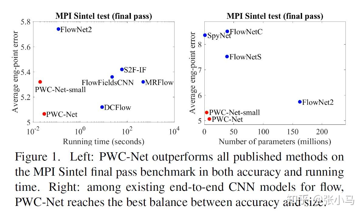
简单说一下号称compact but effective CNN model的光流学习网络PWC-Net[1].
该网络基于三个简单但是由来已久的原则：金字塔式处理（pyramidal processing）；基于上一层习得的光流偏移下一层特征，逐层学习下一层细部光流（warping）；设计代价容量函数（cost volume). 尽管PWC-Net的网络尺寸比flownet2小了17倍（Flownet2需要640MB的memory footprint），也更加容易训练，却在MPI Sintel final pass 和 KITTI 2015 benchmarks表现的最好。


成功关键：
Cost volume: 代价容量存储了两帧图像之间对应像素的匹配代价。其最初的定义适用于stereo matching这一特殊的光流情景。近期有一些改良用于普遍的光流场景，他们基于单一范围，而且computationally expensive and memory intensive.  我们（指作者）重新定义的方法.......(很好就是了)（constructing a partial cost volume at multiple pyramid levels leads to both effective and efficient models. 嗯，真香）
借助于Phil贡献的代码[2]，我们得以窥探其具体实现。
具体的方法

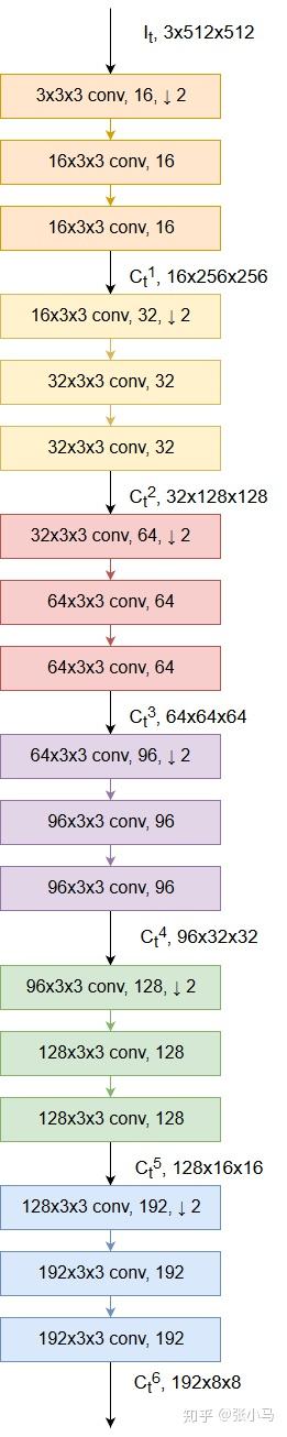
Feature pyramid extractor:

given two input images I1 and I2, we generate L-level pyramids of feature representations, with the bottom (zeroth) level being the input images,  i.e.,  C_t^0= I_t.
To generate feature representation at the l-th layer,  C_t^l , we use layers of convolutional filters to downsample the features at the (l−1)th pyramid level,  C_t^{l-1} , by a factor of 2. From the first to the sixth levels, the number of feature channels are respectively 16, 32, 64, 96, 128, and 196.
Individual images of the image pair are encoded using the same Siamese network. Each convolution is followed by a leaky ReLU unit. The convolutional layer and the x2 downsampling layer at each level is implemented using a single convolutional layer with a stride of 2.

文章配的结构图在每层特征提取的网络里少了一层，所以这里我自己又画了一个。


    def extract_features(self, x_tnsr, name='featpyr'):
        """Extract pyramid of features
        Args:
            x_tnsr: Input tensor (input pair of images in [batch_size, 2, H, W, 3] format)
            name: Variable scope name
        Returns:
            c1, c2: Feature pyramids
        """
        assert(1 <= self.opts['pyr_lvls'] <= 6)
        if self.dbg:
            print(f"Building feature pyramids (c11,c21) ... (c1{self.opts['pyr_lvls']},c2{self.opts['pyr_lvls']})")
        # Make the feature pyramids 1-based for better readability down the line
        num_chann = [None, 16, 32, 64, 96, 128, 196]
        c1, c2 = [None], [None]
        init = tf.keras.initializers.he_normal()
        with tf.variable_scope(name):
            for pyr, x, reuse, name in zip([c1, c2], [x_tnsr[:, 0], x_tnsr[:, 1]], [None, True], ['c1', 'c2']):
                for lvl in range(1, self.opts['pyr_lvls'] + 1):
                    # tf.layers.conv2d(inputs, filters, kernel_size, strides=(1, 1), padding='valid', ... , name, reuse)
                    # reuse is set to True because we want to learn a single set of weights for the pyramid
                    # kernel_initializer = 'he_normal' or tf.keras.initializers.he_normal(seed=None)
                    f = num_chann[lvl]
                    x = tf.layers.conv2d(x, f, 3, 2, 'same', kernel_initializer=init, name=f'conv{lvl}a', reuse=reuse)
                    x = tf.nn.leaky_relu(x, alpha=0.1)  # , name=f'relu{lvl+1}a') # default alpha is 0.2 for TF
                    x = tf.layers.conv2d(x, f, 3, 1, 'same', kernel_initializer=init, name=f'conv{lvl}aa', reuse=reuse)
                    x = tf.nn.leaky_relu(x, alpha=0.1)  # , name=f'relu{lvl+1}aa')
                    x = tf.layers.conv2d(x, f, 3, 1, 'same', kernel_initializer=init, name=f'conv{lvl}b', reuse=reuse)
                    x = tf.nn.leaky_relu(x, alpha=0.1, name=f'{name}{lvl}')
                    pyr.append(x)
        return c1, c2Warping layer:

At the l-th level, we warp features of the second image toward the first image using the x2 upsampled flow from the l+1th level:  C_w^l(x) = C_2^l(x+ up_2(w^{l+1})(x))
where x is the pixel index and the upsampled flow up_2(w^{l+1}) is set to be zero at the top level.
We use bilinear interpolation to implement the warping operation and compute the gradients to the input CNN features and flow for backpropagation according to E. Ilg's FlowNet 2.0 paper.
For non-translational motion, warping can compensate for some geometric distortions and put image patches at the right scale.

The warping and cost volume layers have no learnable parameters and, hence, reduce the model size.
    def warp(self, c2, sc_up_flow, lvl, name='warp'):
        """Warp a level of Image1's feature pyramid using the upsampled flow at level+1 of Image2's pyramid.
        Args:
            c2: The level of the feature pyramid of Image2 to warp
            sc_up_flow: Scaled and upsampled estimated optical flow (from Image1 to Image2) used for warping
            lvl: Index of that level
            name: Op scope name
        """
        op_name = f'{name}{lvl}'
        if self.dbg:
            msg = f'Adding {op_name} with inputs {c2.op.name} and {sc_up_flow.op.name}'
            print(msg)
        with tf.name_scope(name):
            return dense_image_warp(c2, sc_up_flow, name=op_name)

    def dense_image_warp(image, flow, name='dense_image_warp'):
        """Image warping using per-pixel flow vectors.

        Apply a non-linear warp to the image, where the warp is specified by a dense
        flow field of offset vectors that define the correspondences of pixel values
        in the output image back to locations in the  source image. Specifically, the
        pixel value at output[b, j, i, c] is
        images[b, j - flow[b, j, i, 0], i - flow[b, j, i, 1], c].

        The locations specified by this formula do not necessarily map to an int
        index. Therefore, the pixel value is obtained by bilinear
        interpolation of the 4 nearest pixels around
        (b, j - flow[b, j, i, 0], i - flow[b, j, i, 1]). For locations outside
        of the image, we use the nearest pixel values at the image boundary.


        Args:
          image: 4-D float `Tensor` with shape `[batch, height, width, channels]`.
          flow: A 4-D float `Tensor` with shape `[batch, height, width, 2]`.
          name: A name for the operation (optional).

          Note that image and flow can be of type tf.half, tf.float32, or tf.float64,
          and do not necessarily have to be the same type.

        Returns:
          A 4-D float `Tensor` with shape`[batch, height, width, channels]`
            and same type as input image.

        Raises:
          ValueError: if height < 2 or width < 2 or the inputs have the wrong number
                      of dimensions.
        """
        with ops.name_scope(name):
            batch_size, height, width, channels = array_ops.unstack(array_ops.shape(image))
            # The flow is defined on the image grid. Turn the flow into a list of query
            # points in the grid space.
            grid_x, grid_y = array_ops.meshgrid(
                math_ops.range(width), math_ops.range(height))
            stacked_grid = math_ops.cast(
                array_ops.stack([grid_y, grid_x], axis=2), flow.dtype)
            batched_grid = array_ops.expand_dims(stacked_grid, axis=0)
            query_points_on_grid = batched_grid - flow
            query_points_flattened = array_ops.reshape(query_points_on_grid,
                                                       [batch_size, height * width, 2])
            # Compute values at the query points, then reshape the result back to the
            # image grid.
            interpolated = _interpolate_bilinear(image, query_points_flattened)
            interpolated = array_ops.reshape(interpolated,
                                             [batch_size, height, width, channels])
            return interpolatedCost volume layer:

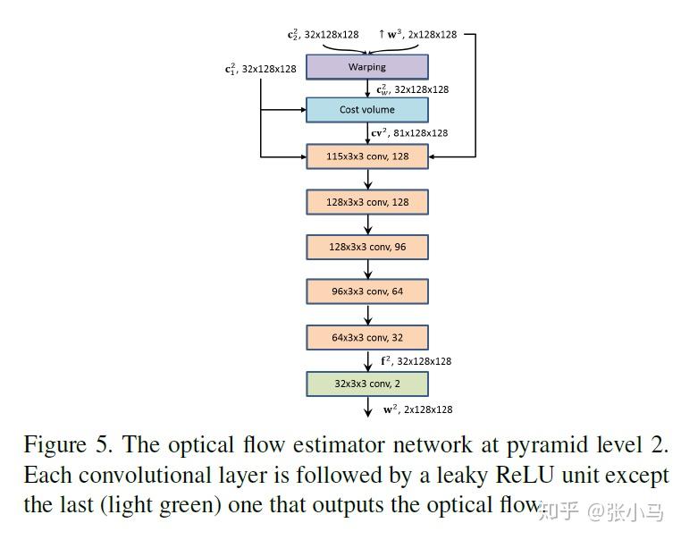
A cost volume stores the data matching costs for associating a pixel from Image1 with its corresponding pixels in Image2. Most traditional optical flow techniques build the full cost volume at a single scale, which is both computationally expensive and memory intensive. By contrast, PWC-Net constructs a partial cost volume at multiple pyramid levels.
The matching cost is implemented as the correlation between features of the first image and warped features of the second image:
CV^l(x1,x2) = \frac{1}{N}(C_1^l(x_1))^T C^l_w(x_2)  
where where T is the transpose operator and N is the length of the column vector C_1^l(x_1) .
For an L-level pyramid, we only need to compute a partial cost volume with a limited search range of d pixels. A one-pixel motion at the top level corresponds to 2^{L-1} pixels at the full resolution images.
Thus we can set d to be small, e.g. d=4. The dimension of the 3D cost volume is d^2\times H^l\times W^l , where H^l  and W^l denote the height and width of the L-th pyramid level, respectively.

The warping and cost volume layers have no learnable parameters and, hence, reduce the model size.

In "Implementation details," we use a search range of 4 pixels to compute the cost volume at each level.
from __future__ import absolute_import, division, print_function
import tensorflow as tf


def cost_volume(c1, warp, search_range, name):
    """Build cost volume for associating a pixel from Image1 with its corresponding pixels in Image2.
    Args:
        c1: Level of the feature pyramid of Image1
        warp: Warped level of the feature pyramid of image22
        search_range: Search range (maximum displacement)
    """
    padded_lvl = tf.pad(warp, [[0, 0], [search_range, search_range], [search_range, search_range], [0, 0]])
    _, h, w, _ = tf.unstack(tf.shape(c1))
    max_offset = search_range * 2 + 1

    cost_vol = []
    for y in range(0, max_offset):
        for x in range(0, max_offset):
            slice = tf.slice(padded_lvl, [0, y, x, 0], [-1, h, w, -1])
            cost = tf.reduce_mean(c1 * slice, axis=3, keepdims=True)
            cost_vol.append(cost)
    cost_vol = tf.concat(cost_vol, axis=3)
    cost_vol = tf.nn.leaky_relu(cost_vol, alpha=0.1, name=name)

    return cost_vol



def corr(self, c1, warp, lvl, name='corr'):
        """Build cost volume for associating a pixel from Image1 with its corresponding pixels in Image2.
        Args:
            c1: The level of the feature pyramid of Image1
            warp: The warped level of the feature pyramid of image22
            lvl: Index of that level
            name: Op scope name
        """
        op_name = f'corr{lvl}'
        if self.dbg:
            print(f'Adding {op_name} with inputs {c1.op.name} and {warp.op.name}')
        with tf.name_scope(name):
            return cost_volume(c1, warp, self.opts['search_range'], op_name)
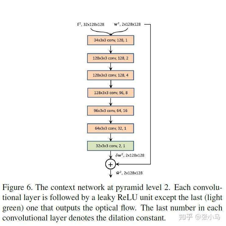
Context network:

Traditional flow methods often use contextual information to post-process the flow. Thus we employ a sub-network, called the context network, to effectively enlarge the receptive field size of each output unit at the desired pyramid level. It takes the estimated flow and features of the second last layer from the optical flow estimator and outputs a refined flow.
The context network is a feed-forward CNN and its design is based on dilated convolutions. It consists of 7 convolutional layers. The spatial kernel for each convolutional layer is 3×3. These layers have different dilation constants. A convolutional layer with a dilation constant k means that an input unit to a filter in the layer are k-unit apart from the other input units to the filter in the layer, both in vertical and horizontal directions. Convolutional layers with large dilation constants enlarge the receptive field of each output unit without incurring a large computational burden. From bottom to top, the dilation constants are 1, 2, 4, 8, 16, 1, and 1.

def refine_flow(self, feat, flow, lvl, name='ctxt'):
        """Post-ptrocess the estimated optical flow using a "context" nn.
        Args:
            feat: Features of the second-to-last layer from the optical flow estimator
            flow: Estimated flow to refine
            lvl: Index of the level
            name: Op scope name
        """
        op_name = f'refined_flow{lvl}'
        if self.dbg:
            print(f'Adding {op_name} sum of dc_convs_chain({feat.op.name}) with {flow.op.name}')
        init = tf.keras.initializers.he_normal()
        with tf.variable_scope(name):
            x = tf.layers.conv2d(feat, 128, 3, 1, 'same', dilation_rate=1, kernel_initializer=init, name=f'dc_conv{lvl}1')
            x = tf.nn.leaky_relu(x, alpha=0.1)  # default alpha is 0.2 for TF
            x = tf.layers.conv2d(x, 128, 3, 1, 'same', dilation_rate=2, kernel_initializer=init, name=f'dc_conv{lvl}2')
            x = tf.nn.leaky_relu(x, alpha=0.1)
            x = tf.layers.conv2d(x, 128, 3, 1, 'same', dilation_rate=4, kernel_initializer=init, name=f'dc_conv{lvl}3')
            x = tf.nn.leaky_relu(x, alpha=0.1)
            x = tf.layers.conv2d(x, 96, 3, 1, 'same', dilation_rate=8, kernel_initializer=init, name=f'dc_conv{lvl}4')
            x = tf.nn.leaky_relu(x, alpha=0.1)
            x = tf.layers.conv2d(x, 64, 3, 1, 'same', dilation_rate=16, kernel_initializer=init, name=f'dc_conv{lvl}5')
            x = tf.nn.leaky_relu(x, alpha=0.1)
            x = tf.layers.conv2d(x, 32, 3, 1, 'same', dilation_rate=1, kernel_initializer=init, name=f'dc_conv{lvl}6')
            x = tf.nn.leaky_relu(x, alpha=0.1)
            x = tf.layers.conv2d(x, 2, 3, 1, 'same', dilation_rate=1, kernel_initializer=init, name=f'dc_conv{lvl}7')

            return tf.add(flow, x, name=op_name)Training loss:

Adds the L2-norm or L1-norm losses at all levels of the pyramid. In regular training mode, the L2-norm is used to compute the multiscale loss.
\mathcal{L}(\Theta)=\sum_{l=l_0}^{L}{\alpha_l}\sum_{x}{\left| w_{\Theta}^l (x)-w_{GT}^l(x)\right|_2+\gamma\left| \Theta \right|_2}
In fine-tuning mode, the L1-norm is used to compute the robust loss.
\mathcal{L}(\Theta)=\sum_{l=l_0}^{L}{\alpha_l}\sum_{x}{(\left| w_{\Theta}^l (x)-w_{GT}^l(x)\right|+\varepsilon)^q+\gamma\left| \Theta \right|_2}

def pwcnet_loss(y, y_hat_pyr, opts):
    """Adds the L2-norm or L1-norm losses at all levels of the pyramid.
    Args:
        y: Optical flow groundtruths in [batch_size, H, W, 2] format
        y_hat_pyr: Pyramid of optical flow predictions in list([batch_size, H, W, 2]) format
        opts: options (see below)
        Options:
            pyr_lvls: Number of levels in the pyramid
            alphas: Level weights (scales contribution of loss at each level toward total loss)
            epsilon: A small constant used in the computation of the robust loss, 0 for the multiscale loss
            q: A q<1 gives less penalty to outliers in robust loss, 1 for the multiscale loss
            mode: Training mode, one of ['multiscale', 'robust']
    Returns:
        Loss tensor opp
      """
    # Use a different norm based on the training mode we're in (training vs fine-tuning)
    norm_order = 2 if opts['loss_fn'] == 'loss_multiscale' else 1

    with tf.name_scope(opts['loss_fn']):
        total_loss = 0.
        _, gt_height, _, _ = tf.unstack(tf.shape(y))

        # Add individual pyramid level losses to the total loss
        for lvl in range(opts['pyr_lvls'] - opts['flow_pred_lvl'] + 1):
            _, lvl_height, lvl_width, _ = tf.unstack(tf.shape(y_hat_pyr[lvl]))

            # Scale the full-size groundtruth to the correct lower res level
            scaled_flow_gt = tf.image.resize_bilinear(y, (lvl_height, lvl_width))
            scaled_flow_gt /= tf.cast(gt_height / lvl_height, dtype=tf.float32)

            # Compute the norm of the difference between scaled groundtruth and prediction
            if opts['use_mixed_precision'] is False:
                y_hat_pyr_lvl = y_hat_pyr[lvl]
            else:
                y_hat_pyr_lvl = tf.cast(y_hat_pyr[lvl], dtype=tf.float32)
            norm = tf.norm(scaled_flow_gt - y_hat_pyr_lvl, ord=norm_order, axis=3)
            level_loss = tf.reduce_mean(tf.reduce_sum(norm, axis=(1, 2)))

            # Scale total loss contribution of the loss at each individual level
            total_loss += opts['alphas'][lvl] * tf.pow(level_loss + opts['epsilon'], opts['q'])

        return total_loss

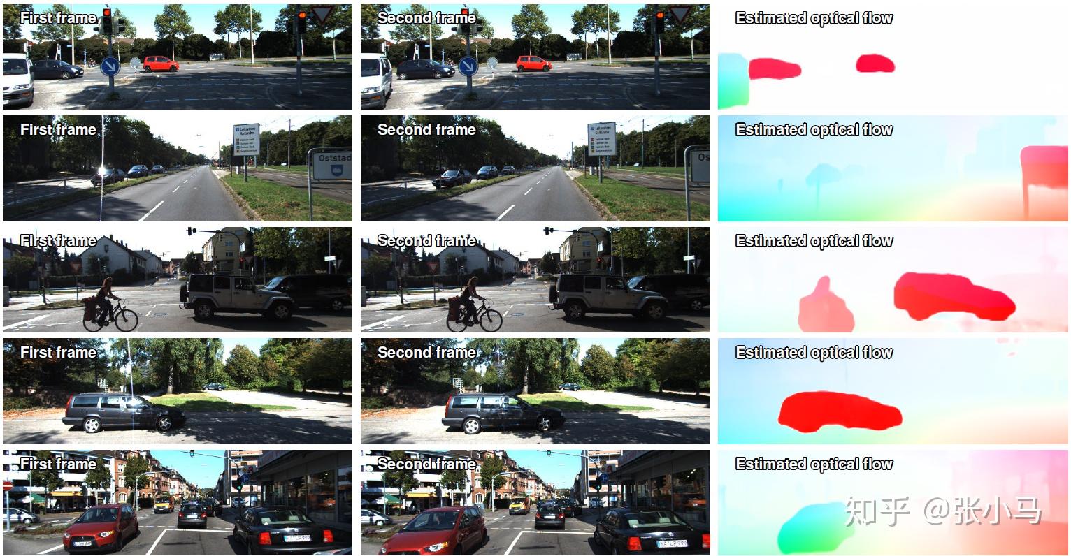
Result



参考

• ^Sun, Deqing, et al. "PWC-Net: CNNs for optical flow using pyramid, warping, and cost volume." Proceedings of the IEEE Conference on Computer Vision and Pattern Recognition. 2018. https://arxiv.org/abs/1709.02371
  
• ^Optical Flow Prediction with Tensorflow https://github.com/philferriere/tfoptflow
  

法戒

加油啊，作者，希望能看到完整的版本。。。

纯属扯淡

我正学习光流提取，太好了，谢谢作者

兔子先森

pwcnet可以用来学习深度吗?

星空迷彩

估计是不行

波嗷宝

这已经很完整了吧……

恨别离

看了半天warp，原来是上采样啊。。。

别忘了我

请问这个wgt是咋计算的呀？

周作斌

作者，您好呀~有关optical flow estimation我到现在还是搞不懂。
cost volumn layer学习了Image-1和Image-2的图像的特征匹配后，与upsampled flow、Image-1的特征作为输入，得到当前的光流图。 我暂时理解为：（*特征匹配后输出的是两图像特征的位移（类似于可变形卷积）， 从而指导upsampled flow进一步完善）；而Image-1的特征则是为纠正（*）所得结果而做输入的。
PS：但是我并不确定[飙泪笑]，如果您有空的话，麻烦回复一个哇~[爱]

邓志刚

是这样的，一边学习位移，一边纠正